What is the Continuity Correction Factor?

What is the Continuity Correction Factor?

Continuity correction factor

Because the normal distribution can take all real numbers (is continuous) but the binomial distribution can only take integer values (is discrete), a normal approximation to the binomial should identify the binonial event "8" with the normal interval "(7.5, 8.5)" (and similarly for other integer values). The figure below shows that for P(X > 7) we want the magenta region which starts at 7.5.

---

---

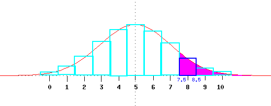
Example: If n=20 and p=.25, what is the probability that X is greater than or equal to 8?

• The normal approximation without the continuity correction factor yields
  z=(8-20 × .25)/(20 × .25 × .75)^.5 = 1.55, hence P(X *greater than or equal to* 8) is approximately .0606 (from the table).
• The continuity correction factor requires us to use 7.5 in order to include 8 since the inequality is weak and we want the region to the right. z = (7.5 - 5)/(20 × .25 × .75)^.5 = 1.29, hence the area under the normal curve (magenta in the figure above) is .0985.
• The exact solution is .1019 approximation

Hence for small n, the continuity correction factor gives a much better answer.

Competencies: Use the normal approximation with the continuity correction factor to approximate the probability of more than 40 successes if n=60 and p=.75.

A continuity correction factor is used when you use a continuous function to approximate a discrete one. For example, when you want to approximate a binomial with a normal distribution. According to the Central Limit Theorem, the sample mean of a distribution becomes approximately normal if the sample size is large enough. Thebinomial distribution can be approximated with a normal distribution too, as long as n*p and n*q are both at least 5.

Continuity Correction Factor Table

If   P(X=n) use   P(n – 0.5 < X < n + 0.5)
If   P(X>n) use   P(X > n + 0.5)
If   P(X≤n) use    P(X < n + 0.5)
If    P (X<n) use   P(X < n – 0.5)
If    P(X ≥ n) use   P(X > n – 0.5)

A numerical example: Toss a fair coin 100$100$ times. Approximate the probability that the number of heads is ≤55$\le 55$.

By working directly with the binomial, and software, I get this is, to 6$6$ figures, 0.864373$0.864373$. That's the "right" answer.

Using Pr(Y≤55)$Pr(Y\le 55)$, where Y$Y$ is normal mean 50$50$, standard deviation 5$5$, no continuity correction, I get the approximation 0.8413$0.8413$.

Using the continuity correction, I get the approximation 0.8643$0.8643$. I should really do a few other examples, the continuity correction is too good here!

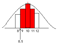
In this diagram, the rectangles represent the binomial distribution and the curve is the normal distribution:

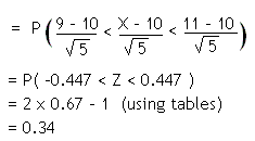
We want P(9 ≤ X ≤ 11), which is the red shaded area. Notice that the first rectangle starts at 8.5 and the last rectangle ends at 11.5 . Using a continuity correction, therefore, our probability becomes P(8.5 < X < 11.5) in the normal distribution.

Standardising

Probability Distributions

Find The Right Fit With Probability Distributions
By David Harper

Probability Distributions are pictures that describe a particular view of uncertainty. 

An emergent research view holds that financial markets are both uncertain and predictable. Also, markets can be efficient but also uncertain. In finance, we use probability distributions to draw pictures that illustrate our view of an asset return's sensitivity when we think the asset return can be considered a random variable. 

There are two ways of categorizing distributions: by whether it is discrete or continuous, and by whether it is a probability density function (PDF) or a cumulative distribution.

The PDF is P[x=X]; The cumulative distribution is P[x<=X]

UniformThe simplest and most popular distribution is the uniform distribution in which all outcomes have an equal chance of occurring.

Now roll three dice together, as shown in Figure 4. We start to see the effects of a most amazing theorem: the central limit theorem.

The central limit theorem boldly promises that the sum or average of a series of independent variables will tend to become normally distributed, regardless of their own distribution. Our dice are individually uniform but combine them and - as we add more dice - almost magically their sum will tend toward the familiar normal distribution! 

Binomial

The binomial distribution reflects a series of "either/or" trials, such as a series of coin tosses. These are called Bernoulli trials but you don't need even (50/50) odds. A Bernoulli trial refers to events that have only two outcomes. 

The binomial distribution below plots a series of 10 coin tosses where the probability of heads is 50% (p-0.5). You can see in Figure 6 that the chance of flipping exactly five heads and five tails (order doesn't matter) is just shy of 25%:

As the number of trials increase, the binomial tends toward the normal distribution.

LognormalThe lognormal distribution is very important in finance because many of the most popular models assume that stock prices are distributed lognormally. It is easy to confuse asset returns with price levels:



http://www.investopedia.com/articles/06/probabilitydistribution.asp